What to Expect in CFA Level 1 Quantitative Methods?
CFA Level 1 Quantitative Methods curriculum covers understanding and interpreting a normal distribution and how it relates to quantifying risk. At 6-9% of the exam, Quantitative Methods is given less weight than Ethics and Financial Statement analysis but is weighted more heavily than most topics. Candidates will also become familiar with data visualization, probability distributions, sampling and estimation, hypothesis testing, and regression analysis.
Exam Weighting
The CFA Quantitative Methods topic weighs 6-9%, meaning that approximately 11-16 of the 180 CFA Level 1 exam questions focus on this topic.
| Topic Weight | No. of Learning Modules | No. of Formulas | No. of Questions |
|---|---|---|---|
| 6-9% | 11 | ca. 100 | ca. 16 |
Level 1 Quantitative Methods 2026 Syllabus, Readings, and Changes
While the CFA Level 1 Quantitative Methods curriculum emphasizes understanding normal distribution, risk quantification, and various topics like data visualization and regression, the latest syllabus introduces new topics like Rates and Returns and Big Data Techniques, reflecting contemporary advancements in financial technology. Despite these updates, the core focus on quantitative analysis remains intact.
Rates and Returns
This topic centers on interpreting interest rates as required rates of return, discount rates, or opportunity costs. It emphasizes calculating and interpreting different return measurement approaches, comparing money-weighted and time-weighted rates of return, and evaluating portfolio performance. Additionally, candidates learn to calculate and interpret annualized return measures, continuously compounded returns, and major return measures with a focus on their appropriate applications.
Time Value of Money
We can express one of the core concepts of the time value of money through an age-old proverb—a bird in the hand is worth two in the bush. How does this relate to finance? Money now is worth more than money later: time imposes risk, which has a cost that detracts from value. Therefore, financial analysts must understand how to factor time into valuation.
This reading covers how to calculate
- the future value of a cash flow or a series of cash flows or
- the present value of a cash flow or series of cash flows happening in the future
Candidates are introduced to terminology and concepts that will curate a sense of economic intuition for material covered in later readings.
Statistical Measures of Asset Returns
This topic delves into the intricate world of financial analysis, where we engage in the calculation, interpretation, and assessment of central tendency and location measures. These crucial statistical tools serve as our compass when navigating the complex landscape of investment problems.
In addition to these fundamental concepts, we venture into dispersion measures, striving to comprehend their significance in the context of investment challenges. Furthermore, our exploration expands to encompass the nuanced understanding and evaluation of skewness and kurtosis, offering us valuable insights into the shape and distribution of investment data.
Lastly, we aim to unlock the potential of interpreting the correlation between two variables. This vital skill empowers us to make informed decisions within the framework of addressing intricate investment issues.
Probability Trees and Conditional Expectations
Involves calculating expected values, variances, and standard deviations, showcasing their application to investment problems. Candidates will also learn to formulate an investment problem as a probability tree and understand the application of conditional expectations in investment contexts. Furthermore, the focus extends to calculating and interpreting updated probabilities in investment settings using Bayes’ formula.


Portfolio Mathematics and Simulation Methods
Prospective candidates are required to demonstrate proficiency in several essential quantitative finance skills. These include the ability to calculate and interpret expected values, variances, standard deviations, covariances, and correlations of portfolio returns. Additionally, candidates are expected to possess a comprehensive understanding of risk management, encompassing the definition and evaluation of shortfall risk, the calculation of the safety-first ratio, and the identification of an optimal portfolio through the application of Roy’s safety-first criterion.
Within the realm of Simulation Methods, candidates will acquire the knowledge and expertise necessary to elucidate the normal-lognormal relationship and its significance in modeling asset prices. Furthermore, they will gain proficiency in articulating the principles behind Monte Carlo simulation and mastering the utilization of bootstrap resampling in the context of investment applications.
Hypothesis Testing
Analysts sift through an avalanche of data to assess the investment environment and develop hypotheses. To test these hypotheses, analysts will employ statistical inference, allowing them to make judgments about populations based on smaller sample sizes.
- The reading discusses the three quantities commonly used in investments (mean, variance, and correlation) via a hypothesis-testing framework.
Simple Linear Regression
The process of determining relationships between variables is an important tool in the analyst’s toolkit. One of these tools is regression analysis.
- The reading explains the assumptions underlying the simple linear regression model and the roles of independent variables within that model.
- Candidates will also learn to formulate various hypotheses using this tool.
Parametric and Non-Parametric Tests of Independence
This section explains parametric and nonparametric tests concerning the hypothesis that the population correlation coefficient equals zero. Candidates will determine whether the hypothesis is rejected at a specified level of significance. Furthermore, the topic includes explaining tests of independence based on contingency table data.
Introduction to Big Data Techniques
Introduced this year in this topic, the segment covers describing aspects of “fintech” relevant for gathering and analyzing financial data. Candidates will delve into descriptions of Big Data, artificial intelligence, and machine learning. Additionally, the focus extends to describing applications of Big Data and Data Science in the context of investment management.
CFA Quantitative Methods Level 1 Sample Questions and Answers
The sample questions are typical of the probing multiple-choice questions on the L1 exam. During the exam, you have about 90 seconds to read and answer each question, carefully designed to test knowledge from the CFA Curriculum. UWorld’s question bank is built to expose you to exam-like questions and illustrate and explain the concepts tested thoroughly.
An analyst determines that the probabilities of two events are as follows:
| Event | Description | Probability |
|---|---|---|
| A | Price of oil increases | 0.33 |
| B | S&P 500 Index increases | 0.49 |
Assuming the events are independent but not mutually exclusive, the probability that at least one of the two events will occur is closest to:
- 0.16
- 0.66
- 0.82
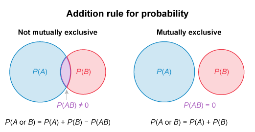
The probability that at least one of the two events ( A or B) will occur is the same as the probability that:
- Only A ( one event ) will occur, or
- Only B ( one event ) will occur, or
- Both A and B ( two events ) will occur.
The addition rule for probability states that for events that are not mutually exclusive:
P( A or B) = P(A) + P(B) − P(AB)
Note that the probability that both events occur, which is possible since the events are not mutually exclusive, must be subtracted to avoid double counting that probability.
In this scenario, P(A) and P(B) are given, but the probability of both A and B [ P( AB) ] is not given. However, for independent events, P(AB) can be calculated according to the multiplication rule for probability as P(A) P(B). Substituting P(A) P(B) for P(AB) into the addition rule above:
P(A or B) = P(A) + P(B) − P(A) P(B)
= 0.33 + 0.49 − (0.33 × 0.49)
= 0.6583 ≈ 0.66, or 66%
(Choice A) 0.1617 is the result of multiplying P(A) and P(B). This is P(AB), the probability that both A and B will occur, not the probability of A or B.
(Choice C) 0.8200 is the result of treating A and B as mutually exclusive and not subtracting the probability that both events will occur, P(AB). This has the effect of double-counting the probability of A and B both occurring and so overestimates the probability of A or B occurring.
Things to remember:
The addition rule for probability states that for two events that are not mutually exclusive, such as A and B in this scenario, P(A or B) = P(A) + P(B) − P(AB). For independent events, the multiplication rule for probability states that P(AB) = P(A) P(B).
A researcher formulates a null hypothesis stating that a country’s average inflation is 2%. After testing a sample, the researcher fails to reject the null hypothesis when the actual average inflation is not 2%. This most likely results in a:
- Type I error.
- Type II error.
- correct decision.
| Actual Situation | ||
|---|---|---|
| Decision from statistical test | Null (H0) is true | Null (H0) is false |
| Do not reject null (H0) | Correct decision | Type II error |
| Reject null (H0), accept alternative (Ha) | Type I error | Correct decision |
Hypothesis testing involves a decision regarding whether to reject a null hypothesis (H0) based on statistical tests. In this question, the null hypothesis states that the country’s average inflation is 2% (H0: μ = 2%). Conversely, the alternative hypothesis states that the country’s average inflation is not 2% (Ha: μ ≠ 2%).
There are two types of errors that can result from the decision to reject or to not reject the null hypothesis:
- Type I error: Rejecting the null hypothesis when it is true
- Type II error: Failing to reject the null hypothesis when it is false
Here, the null hypothesis is false since actual average inflation is not 2%. Failing to reject the false null hypothesis in this case results in a Type II error.
(Choice A) A Type I error results from rejecting a null hypothesis when it is true. An example of a Type I error would be the analyst rejecting the null hypothesis (H0: μ = 2%) when the actual average inflation is 2%.
(Choice C) Given the actual situation that the average inflation is not 2% (ie, the null hypothesis is false), the correct decision is to reject the null hypothesis (H0: μ = 2%).
Things to remember:
A Type I error results from rejecting the null hypothesis when it is true. A Type II error results from failing to reject the null hypothesis when it is false.
If a cumulative distribution function of a random variable indicates that P(X < a) is equal to P(X ≤ a), then the distribution is most likely :
- normal.
- discrete.
- binomial.
The value of a cumulative distribution function (CDF) for a random variable X is the probability that the variable takes on values less than or equal to a given value a: P(X ≤ a ). The CDF’s values range from 0 to 1 since there is a 100% chance that the random variable takes on values less or equal to its greatest value and the value of the distribution is “cumulative.”
A normal distribution is a continuous distribution. There are an uncountable number of possible outcomes in a continuous distribution, so the probability of a continuous random variable being equal to any one point, P(X = a), is zero. Then:
| P(X ≤ a ) | = P(X < a ) + P(X = a ) |
| = P(X < a ) + 0 | |
| = P(X < a ) |
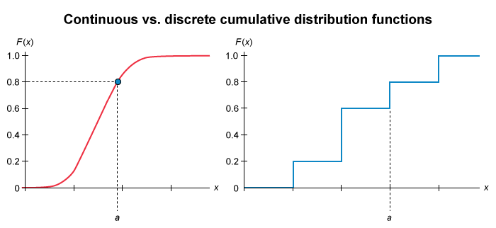
This is illustrated in the image shown above. The CDF of a continuous distribution (red line in the left graph) is smooth.
- For this continuous distribution, P(X < a) = 0.80, while P(X ≤ a) = 0.80, and thus P(X < a ) = P(X ≤ a ).
However, a discrete probability distribution involves a countable number of outcomes, so its CDF resembles a stairstep pattern (blue line in the graph on the right).
- For the discrete distribution, P(X < a) = 0.60, while P(X ≤ a) = 0.80, and thus P(X < a) ≠ P(X ≤ a).
(Choice B) In a discrete distribution, P(X < a) ≠ P(X ≤ a).
(Choice C) The binomial distribution is a type of discrete distribution, so P(X < a) ≠ P(X ≤ a).
Things to remember:
There are an uncountable number of possible outcomes in a continuous distribution, so the probability of a continuous random variable being equal to any one point, P(X = a), is zero. Thus, P(X < a) = P(X ≤ a) for all continuous distributions, such as the normal distribution.
What to Expect in CFA Level 2 Quantitative Methods?
CFA Level 2 Quantitative Methods builds on the material covered in Level 1 while emphasizing hypothesis testing. At 5-10% of the exam, Quantitative Methods is one of the less heavily weighted topics. Candidates will become familiar with tools used to identify relationships among variables and examine fintech, machine learning, and sentiment analysis related to developing an investment hypothesis.
Exam Weighting
The CFA Quantitative Methods topic has a weight of 5-10% of the total exam content, so approximately 4-8 of the 88 CFA Level 2 exam questions, or 1-2 of the 22 item sets focus on this topic.
| Topic Weight | No. of Learning modules | No. of Formulas | No. of Questions |
|---|---|---|---|
| 5-10% | 7 | ca. 50 | ca. 4-8 |
Level 2 Quantitative Methods 2026 Syllabus, Readings, and Changes
The CFA Level 2 Quantitative Methods syllabus covers 7 learning modules, constituting approximately 14.3% of the total curriculum. Notably, several readings have either been consolidated into a single reading or diversified into two or more distinct readings for enhanced comprehension and coverage.
Basics of Multiple Regression and Underlying Assumptions
Financial analysts typically work with sophisticated statistical models that involve more than one independent variable. For example, analysts may want to assess particular macroeconomic variables behind the demand for an individual company’s products or services. To make such assessments, analysts employ multiple linear regression (linear regression with more than one independent variable) to make such assessments.
- The reading introduces the core principles and models of multiple regression models and the foundational assumptions applied to and adjusted for real-world situations.
- Candidates will learn to diagnose an assumption violation and to adjust to these violations.
- The reading also dives into the role of logistic regression in machine learning for Big Data analysis.
Evaluating Regression Model Fit and Interpreting Results
The reading helps understand:
- How well a multiple regression model explains the dependent variable by analyzing ANOVA table results and measures of goodness of fit
- The hypotheses on the significance of two or more coefficients in a multiple regression model and interpret the results of the joint hypothesis tests
- The Calculation and interpretation of a predicted value for the dependent variable, given the estimated regression model and assumed values for the independent variable
Model Misspecification
The reading helps understanding:
- How model misspecification affects the results of a regression analysis and how to avoid common forms of misspecification
- The types of heteroskedasticity and how it affects statistical inference
- Serial correlation and how it affects statistical inference
- Multicollinearity and how it affects regression analysis
Extensions of Multiple Regression
Financial analysts commonly utilize advanced statistical models that incorporate multiple independent variables. One such application involves evaluating specific macroeconomic factors that influence the demand for a company’s products or services. To perform these assessments effectively, analysts rely on the technique known as multiple linear regression, which enables the analysis of relationships between multiple independent variables and a dependent variable. This comprehensive approach is explored through four dedicated learning modules, each delving into the intricate aspects of multiple regression analysis, including:
- The core principles and models of multiple regression models and the foundational assumptions applied to and adjusted for real-world situations.
- The diagnosis of an assumption violation and relevant adjustments.
- The role of logistic regression in machine learning for Big Data analysis.
Time-Series Analysis
A set of these progressive observations is known as a time series, for example, a company’s quarterly sales over three years.
- The reading explores the two fundamental uses of time-series models: understanding the past and forecasting the future of a time series.
- Candidates will learn to estimate time-series models and how these models explain the changes in a time series over time.
Machine Learning
Since their introduction in the 1990s, machine learning techniques have become an integral tool in the toolkits of investment firms. Machine learning (ML) aids analysts in discovering new sources of value and efficiently executing trades.
- The reading provides an overview of machine learning and essential machine learning algorithms applied to investing.
- Candidates will learn about unsupervised machine learning algorithms, neural networks, deep learning nets, and how to choose an appropriate ML algorithm for the task.
Big Data Projects
Big data is an umbrella term that refers to data generated by organizations (businesses, financial markets, governments), individuals (credit cards, social media), sensors, and the Internet of Things. The true impact of big data on financial analysis is yet to be fully understood, but it has already become an integral part of analysts’ toolkits. Data can aid analysts in developing their hypotheses, and forecasting trends in asset prices, detecting anomalies, etc.
- Candidates will learn about the concepts that allow analysts to make predictions using structured and unstructured data.
- The reading provides a real-world ‘big data’ project case study that uses sentiment analysis to assess stock movements.
CFA Quantitative Methods Level 2 Sample Questions and Answers
The sample questions here are typical of the L2 exam’s complexity and depth: formatted as item sets, with a vignette to deliver a scenario that tests the CFA L2 Curriculum. (On the actual exam, each vignette applies to four questions; we’ve thrown in a couple extra to learn more). And be sure to review the illustrated explanations we’ve provided for each question: UWorld’s question bank is designed to expose you to exam-like questions and explain the concepts tested thoroughly.
Passage
Jae Park, CFA, is a manager of a hedge fund that bases its security selection on advanced quantitative analysis. For several open job positions with the fund, Park is looking to hire people with scientific and research backgrounds. Using multiple regression, she would like to evaluate the relationship between the expected salary of the candidates based on their years of experience (EXP), number of published research papers (PRP), and amount of grant funding received in their career (GF). The results of that regression are shown below, along with sample critical values. Park wishes to test the results at a 5% significance level (α = 0.05).
Park also notices that each candidate attended one of five universities. She is considering how to add a variable for university attended to the regression model and believes dummy variables are the best way to capture this.
Finally, Park suspects that her regression in its current form may violate regression assumptions. Her concern is tha ther model might have an artificially large R2 and t-statistics that are understated.
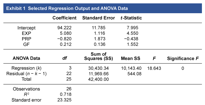
Based on the data in Exhibit 1, the regression is most likely a good predictor of projected salary since:
- it has a high R 2
- the F – statistic has a low p – value.
- most coefficients are statistically significant.
| Exhibit 1 Selected Regression Output and ANOVA Data | |||||
|---|---|---|---|---|---|
| Coefficient | Standard Error | t – Statistic | |||
| Intercept | 94.222 | 11.785 | 7.995 | ||
| EXp | 5.080 | 1.116 | 4.550 | ||
| PRP | -0.820 | 1.873 | -0.438 | ||
| GF | 0.212 | 0.136 | 1.552 | ||
| ANOVA Data | df |
Sum of Squares (SS) |
Mean SS | F | Significance F |
| Regression (k ) | 3 | 30,430.34 | 10,143.40 | 18.643 | 0 |
| Residual (n – k – 1 ) | 22 | 11,969.66 | 544.08 | ||
| Total | 25 | 42,400.00 | |||
| Observations | 26 | ||||
| R 2 | 0.718 | ||||
| Standard error | 23.325 | ||||
Hypothesis testing verifies whether a regression is a good predictor of the dependent variable. Testing can be performed on coefficients or the overall regression.
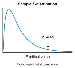
The F-statistic is used to test whether the overall regression (ie, the combination of all slope coefficients) is statistically significant. The null hypothesis (H0) states that the model has no statistically significant coefficients, while the alternative hypothesis (Ha) states that at least one coefficient is significant.
The ANOVA table provides the F – statistic’s p-value ( labeled “significance F ” ). H0 is rejected if the p – value is less than the level of significance (α). In this scenario, the p – value is less than α (0 < 0.05), so H0 is rejected and the regression is statistically significant. In other words, the regression is a good predictor of the dependent variable.
(Choice A) R2 gauges how closely the data fit the regression line. Adding independent variables will increase R2, even if those variables are only slightly correlated with the dependent variable. Furthermore, R2 does not measure statistical significance. Models may have multiple coefficients without statistical significance and still have a high R2. The model’s predictive power depends mainly on the statistical significance of the regression and the coefficients.
(Choice C) A t– test can determine if a slope coefficient is statistically significant. However, the model’s overall fit cannot be determined from t– tests due to possible interactions among the independent variables. Individual coefficients can be statistically significant, but the overall regression is not.
Things to remember:
The F– statistic is used to test how well the regression explains the dependent variable. The null hypothesis H0 states that none of the coefficients are statistically significant, and it can be rejected if the p – value of the F – statistic is less than α. Rejecting H0 indicates that the model is a statistically significant predictor of the dependent variable.
According to Exhibit 1, the most appropriate interpretation of the coefficients is that a higher expected salary will result from:
- more published papers and less grant funding.
- more published papers and more grant funding.
- fewer published papers and more grant funding.
| Exhibit 1 Selected Regression Output and ANOVA Data | |||||
|---|---|---|---|---|---|
| Coefficient | Standard Error | t – Statistic | |||
| Intercept | 94.222 | 11.785 | 7.995 | ||
| EXP | 5.080 | 1.116 | 4.550 | ||
| PRP | -0.820 | 1.873 | -0.438 | ||
| GF | 0.212 | 0.136 | 1.552 | ||
| ANOVA Data | df |
Sum of Squares (SS) |
Mean SS | F | Significance F |
| Regression (k ) | 3 | 30,430.34 | 10,143.40 | 18.643 | 0 |
| Residual (n – k – 1 ) | 22 | 11,969.66 | 544.08 | ||
| Total | 25 | 42,400.00 | |||
| Observations | 26 | ||||
| R 2 | 0.718 | ||||
| Standard error | 23.325 | ||||
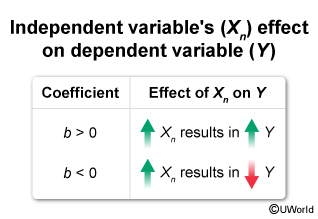
The predicted value of the dependent variable can be derived using the relationship expressed in the regression equation. The slope coefficients of the equation explain the change in the dependent variable, given a one-unit change to one of the independent variables.
The sign of the coefficient indicates the direction of the change in the dependent variable. If the sign of the coefficient is:
- positive, then the independent and dependent variables will move in the same direction.
- negative, then the independent and dependent variables will move in opposite directions.
In this scenario, the PRP and GF coefficients determine how changes to those variables affect the expected salary:
- The PRP coefficient is negative, so a higher PRP variable results in a lower projected salary (Choice A).
- The GF coefficient is positive, so a higher GF variable results in a higher projected salary (Choice B).
Thus, a higher salary would be expected from fewer published papers and more grant funding.
Things to remember:
The sign of a slope coefficient indicates how a change in an independent variable affects the dependent variable.
If a coefficient has a positive sign, then the independent and dependent variables move in the same direction. If a
coefficient has a negative sign, then the independent and dependent variables move in opposite directions.
Based on Exhibits 1 and 2, which slope coefficient is most likely to be statistically significant?
- GF
- EXP
- PRP
| Exhibit 1 Selected Regression Output and ANOVA Data | |||||
|---|---|---|---|---|---|
| Coefficient | Standard Error | t – Statistic | |||
| Intercept | 94.222 | 11.785 | 7.995 | ||
| EXP | 5.080 | 1.116 | 4.550 | ||
| PRP | -0.820 | 1.873 | -0.438 | ||
| GF | 0.212 | 0.136 | 1.552 | ||
| ANOVA Data | df |
Sum of Squares (SS) |
Mean SS | F | Significance F |
| Regression (k ) | 3 | 30,430.34 | 10,143.40 | 18.643 | 0 |
| Residual (n – k – 1 ) | 22 | 11,969.66 | 544.08 | ||
| Total | 25 | 42,400.00 | |||
| Observations | 26 | ||||
| R 2 | 0.718 | ||||
| Standard error | 23.325 | ||||
| Exhibit 2 Sample Values from t -Distribution Table | ||||
|---|---|---|---|---|
| Significance – Two-tailed | 0.100 | 0.050 | ||
| Significance – One-tailed | 0.050 | 0.025 | ||
| df | ||||
| 21 | 1.7207 | 2.0796 | ||
| 22 | 1.7171 | 2.0739 | ||
| 23 | 1.7139 | 2.0687 | ||
| 24 | 1.7109 | 2.0639 | ||
| 25 | 1.7081 | 2.0595 | ||
In a regression model, the slope coefficients describe how a change in an independent variable affects the dependent variable. A t– test is used to verify whether a coefficient meaningfully describes the relationship between an independent and dependent variable.
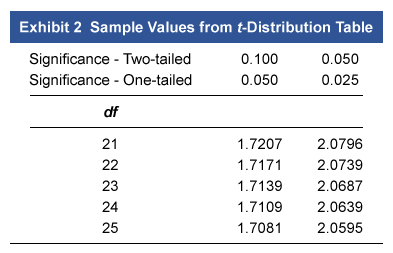
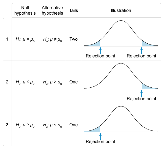
The test seeks to determine whether a coefficient is statistically different from zero. The null hypothesis (H0) states that the coefficient equals zero, while the alternative hypothesis (Ha) states that the coefficient is not equal to zero. The test is also two-tailed, as shown in the image above.
The test compares the t– statistic (t) to the critical value (tc ), and the null is rejected if the absolute value of the t– statistic is greater than the critical value (ie, reject H0 if |t| > tc ). Rejection of H0 means that the coefficient is statistically different from zero (ie, statistically significant).
The steps for the t– test on each of the coefficients are as follows:
| Steps | Calculations |
|---|---|
| Solve for the residuals’ degrees of freedom |
df = n – k – 1 = 26 – 3 – 1 = 22 |
| Solve for the critical t – value | Critical value for 2-tailed test, df = 22, and 5% significance = 2.0739 |
| Compare each t – statistic to the critical value; reject H0 if |t | > tc |
EXP: |4.550| > 2.0739; reject H0 PRP: |-0.438 | < 2.0739; cannot reject H0 GF: |1.552 | < 2.0739; cannot reject H0 |
The null hypothesis is rejected only for EXP. Therefore, EXP is the only statistically significant coefficient; PRP and GF are not statistically significant (Choices A and C).
Things to remember:
The t– test is used to assess whether a slope coefficient is statistically significant. A t– test assumes a null hypothesis where the coefficient equals zero. If the null hypothesis is rejected, then the coefficient is not equal to zero and is therefore statistically significant.
What to Expect in CFA Level 3 Quantitative Methods?
Study Tips for CFA Quantitative Methods
-
Create a Solid Foundation
Because they will come up regularly as you move through the curriculum, Quantitative Methods subjects are fundamental knowledge you need to study closely. Candidates can expect to refer back to these readings for refreshers throughout the exam process.
-
Lots of Practice and Repetition
CFA Institute suggests the importance of practice, particularly the CFA quant section. UWorld’s Qbank provides over 425 individual questions and explanations (from Level 1 and Level 2) to help you gain fluency with quantitative concepts and practice. Answering as many questions as possible can significantly aid in your grasp of the concepts and the exam's testing formats.
-
Start your studies (early) with Quantitative Methods
The order of topics is a common question with most candidates. It is a good idea to start with Quantitative Methods, or at least learn it early in your preparation. These readings introduce fundamental concepts that make up the Level 1 syllabus and that you must grasp to do well on exam day. Additionally, as you go toward your CFA charter, this content will recur throughout the program at every level.
-
Prioritize the rationale over memorization of the formula
You would do well to become very familiar with a number of the equations; you'll probably use your calculator a lot when responding to questions on this subject. However, mastering this content involves more than just crunching numbers. While it is important to apply the concepts, it’ll be easier to recall how to do that if you understand the context as well. In some cases, if you really understand the concepts, you won’t have to rely on your calculator at all.
-
Level 2 is more conceptual than Level 1, but you’ll still have to do the math
Level 2 Quantitative Methods is more: more complex models, more variables, more formulae, but also more theory and understanding of why the math works. But you will still have to crunch the numbers.
-
Put the time in understanding and practicing your itemset/vignette exam technique
Quant is a great place to misread and misuse numbers, so be sure you have a plan for reading through the vignette and then doubling back to find the necessary data—and to ignore the unnecessary data—as you answer specific questions. Always be aware of what the vignette does and doesn’t give you.
-
Be sure to master calculator functions
During the exam, you don’t want to be wishing that you had paid more attention to learning the calculator functions. They can be a huge time saver, keeping you from fumbling and wasting time. And anyways, these are skills that will always come in handy.
For more information, visit our CFA Level 1 Study Schedule, Level 2 Study Schedule and Level 3 Study Schedule


Frequently Asked Questions
Is the Quantitative Method topic hard?
Quantitative Methods is one of the more difficult topics in the CFA Level 1 and Level 2 curriculum, since it is often the least familiar. Candidates who have not had much exposure to quantitative techniques and concepts may have a harder time with this topic.
How can I study Quantitative Methods for the CFA exam?
The CFA Quant section is the most formula-driven and mathematical. It is also significant in the CFA exam at the first two levels, accounting for 12% of the exam at Level 1 and 5-10% of the Level 2 exam. But the knowledge really carries over into all sections of the curriculum, so candidates must understand the fundamentals of Quantitative Methods at Level 1. People learn quantitative ideas differently, but it’s always best to practice, practice, practice.
How do I practice for the CFA Quantitative Methods topic?
The best method, after reviewing the CFA Institute curriculum, is to adopt an active learning approach. But don’t just take our word for it. Give us a try and discover for yourself what it’s like to experience active learning with UWorld’s extensive Level 1 Qbank and with our Level 2 Qbank.
What topics are included in the CFA Quantitative Methods syllabus?
The CFA Quantitative Methods syllabus includes time value of money, discounted cash flow applications, descriptive statistics, probability concepts, common probability distributions, sampling and estimation, hypothesis testing, correlation and covariance, basic portfolio mathematics, and at Level 2, multiple regression, time-series analysis, and machine learning fundamentals.
How many Quantitative Methods questions appear on the CFA exam?
Quantitative Methods typically represent 6–9% of the Level 1 exam and 5–10% of the Level 2 exam. The number of questions varies by cycle, but candidates should expect several item sets or question groups that test both conceptual understanding and formula application.
What is the difference between Quantitative Methods in Level 1 and Level 2?
Level 1 focuses on foundational quantitative tools such as time value of money, probability, common distributions, hypothesis testing, and basic portfolio math, while Level 2 introduces deeper analytical methods including multiple regression, time-series forecasting, machine learning concepts, and advanced statistical interpretation required for investment analysis.
Do Quantitative Methods appear in CFA Level 3?
Quantitative Methods does not appear as a stand-alone topic at Level 3, but its concepts—such as regression outputs, risk measures, returns forecasting, and statistical interpretation—are integrated into Portfolio Management and Wealth Management readings and can appear in both item sets and essay-style problems.
Do I need a strong math background for CFA Quantitative Methods?
A strong math background is helpful but not required. The curriculum teaches all necessary quantitative tools, and most concepts rely on understanding logic rather than advanced mathematics. Basic comfort with algebra, statistics, and using a financial calculator makes learning the material easier.
What formulas are most important in CFA Quantitative Methods?
Key formulas include time value of money equations, probability rules, expected return and variance, correlation and covariance, confidence intervals, test statistics for hypothesis testing, and at Level 2, regression coefficients, R-squared, F-statistics, and Durbin-Watson metrics.
What is the best way to memorize formulas for CFA Quantitative Methods?
The most effective way to memorize formulas is to understand how each formula works, practice applying them to different question types, and reinforce retention using formula sheets or flashcards such as UWorld’s SimpleSheets and ReadyDeck flashcards.
Is a calculator required for CFA Quantitative Methods?
Yes. Many Quantitative Methods questions require a CFA-approved calculator such as the BA II Plus or HP 12C. Candidates must be comfortable performing time value of money calculations, cash flow analysis, probability functions, and basic statistical operations using their calculator. Check the CFA exam calculator page for more information.

