Fixed income instruments offer a broad spectrum of utility, serving investors and issuers with purposes ranging from income generation and safeguarding of principal to intricate asset-liability management. Notably, the credit risk assessment associated with fixed-income securities has gained profound significance since the aftermath of the global financial crisis 2008.
| Fixed Income | ||
|---|---|---|
| Topic Weight | Number of Questions | |
| Level 1 | 11-14% | 20-25 |
| Level 2 | 10-15% | Ca. 11 |
The Fixed Income segment of the curriculum is known for its quantitative nature, and it ranks among the more challenging areas covered in the CFA exam. Its prominence is sustained throughout all 3 levels, making it a pivotal component of the CFA program. Within this subject matter, you are introduced to an extensive array of financial concepts and formulas that are indispensable for proficient financial analysis, whether within the purview of fixed income or in broader financial contexts.
What to Expect in CFA Level 1 Fixed Income
On the CFA Institute’s Level 1 exam, Fixed Income is among the top 3 most heavily weighted topics, along with Financial Statement Analysis and Ethics.
You are taught to define fixed income securities and calculate and interpret their associated features. The material covers securitization, the fundamentals of credit risk, and the influence of interest rates on bond returns
Exam Weighting
The CFA Fixed Income topic has a weight of 11-14% of the total exam content, so that approximately 20-25 of the 180 CFA Level 1 exam questions focus on this topic.
| No. of Learning Modules | No. of Formulas |
|---|---|
| 19 | ca. 40 |
Level 1 Fixed Income 2026 Syllabus, Readings, and Changes
TheCFA Level 1 curriculum has about 19 readings for Fixed Income (8.2% of the total curriculum).
| No. of Learning Modules – 19 | No. of LOS – 51 | |
|---|---|---|
|
Summary
The learning modules introduce attributes of various Fixed Income securities and how to calculate and interpret bond prices, yields, and spreads, and then also introduces securitization and provides an overview of global debt markets. The material covers fundamentals of bond returns and risks with special attention given to interest rates and credit risk. It also introduces key factors for assessing bond sensitivity and credit analysis.
|
||
Fixed-Income Instrument Features
The focus of the topic is on understanding fixed-income instruments, encompassing the description of their features. Additionally, you are expected to delve into the contents of a bond indenture, emphasizing the ability to contrast affirmative and negative covenants.
Fixed Income Markets: Issuance and Trading
Global Fixed Income markets include publicly traded securities and non-publicly traded loans. These markets typically attract less attention despite being 3 times larger than global equity markets.
The learning module presents a summary of global fixed income markets and their major players. You will be introduced to fixed income indexes and fixed income trading in secondary markets.
Fixed-Income Cash Flows and Types
This topic focuses on comprehending fixed-income cash flows and types. This involves describing the common cash flow structures of fixed-income instruments and contrasting cash flow contingency provisions that benefit issuers and investors. Additionally, you are expected to articulate how legal, regulatory, and tax considerations impact the issuance and trading of fixed-income securities.
Fixed-Income Markets for Corporate Issuers
Many kinds of assets generate cash flows for their investors, such as mortgages, auto loans, student loans, bank loans, etc. When those cash flows are securitized, they pass through an entity that repackages them as fixed income securities, and their cash flows become the basis of that asset’s value. Special entities issue these securities as asset-backed securities (ABS).
You will be introduced to the benefits of securitization for investors, issuers, economies, and financial markets. The learning module also explores the various characteristics of different ABS types and their associated risks.
Fixed-Income Markets for Government Issuers
The focus of this topic is on understanding funding choices made by sovereign and non-sovereign governments, quasi-government entities, and supranational agencies. You are expected to describe these funding choices. The topic also involves contrasting the issuance and trading of government and corporate fixed-income instruments.
Yield and Yield Spread Measures: Fixed Rate Bonds and Floating Rate Instruments
The focus of this section is on the ability to calculate the annual yield on a bond for varying compounding periods within a year. Additionally, you are expected to compare, calculate, and interpret yield and yield spread measures for fixed-rate bonds. Similarly, in the context of yield and yield spread measures for floating-rate instruments, the emphasis is on the capability to calculate and interpret yield spread measures for such instruments and calculate and interpret yield measures specifically tailored for money market instruments.
Fixed-Income Risk and Credit Analysis (An Overview)
This section covers essential concepts in fixed-income risk and credit analysis:
| Yield-Based Bond Measures |
|
| Yield-Based Bond Convexity and Portfolio |
|
| Curve-Based and Empirical Risk Measures |
|
| Credit Risk |
|
| Credit Analysis for Government and Corporate Issuers |
|
| Fixed-Income Securitization |
|
CFA Fixed Income Level 1 Sample Questions and Answers
These sample questions are typical of the probing multiple-choice questions on the CFA L1 exam. During the exam, you have about 90 seconds to read and answer each question, carefully designed to test knowledge from the CFA curriculum. UWorld’s question bank is built to expose you to exam-like questions and illustrate and explain the concepts tested thoroughly.
An analyst has gathered the following information on zero-coupon government bond yields:
| Maturity | Spot Rate |
|---|---|
| 1 year | 2.42% |
| 2 years | 3.05% |
| 3 years | 3.48% |
| 4 years | 3.65% |
If the rates are based on a periodicity of 1, the one-year forward rate 2 years in the future (2y1y) is closest to:
- 3.72%
- 4.16%
- 4.35%
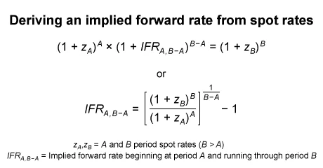
A forward rate (or implied forward rate [IFR]) is a future period interest rate. Forward rates are not expectations of future spot rates; instead, they are future interest rates that reflect the difference between spot rates of different maturities (ie, tenors), based on the assumption that investment strategies covering the same time horizon and carrying equivalent risk should have the same return. In effect, forward rates are the breakeven reinvestment rates that produce that result. Arbitrage-free pricing enforces the consistency of forward rates with spot rate differences.
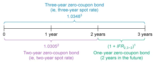
In this scenario, equal amounts invested in a strategy today should have the same future value at the end of 3 years. To answer this question, two investment strategies can be compared as follows:
- Buy a three-year zero-coupon bond and hold it to maturity (ie, right side of the first equation above).
- Buy a two-year zero-coupon bond and hold it to maturity; at maturity, reinvest the proceeds in a one-year zero-coupon bond (ie, left side of the first equation above).
These two strategies are illustrated on the following timeline:
The IFR for the one-year forward rate starting 2 years in the future (IFR2,3−2) is calculated as follows:

(Choice A) 3.72% results from incorrectly calculating the IFR as [(1 + Three-year spot rate)3 − 1] / 2.
(Choice B) 4.16% is the one-year forward rate starting 3 years in the future.
Things to remember:
A forward rate is a future period interest rate that reflects the difference between spot rates of different tenors. In effect, forward rates are breakeven reinvestment rates that result in two investment strategies of equivalent risk, covering the same time horizon and earning the same return.
A two-year floating-rate note pays three-month Libor plus 15 basis points. The floater is priced at 99.60 per 100 par value, three-month Libor is currently 1.45%, and the coupon reset today. Assuming a 30/360 day-count convention and quarterly coupon payments, the discount margin in basis points (bps) is closest to:
- 35 bps
- 40 bps
- 45 bps
A floating-rate note (FRN) is a debt instrument with an interest rate that resets periodically, so that the interest rate and payments are “floating” and not fixed. The interest rate is based on a reference rate, such as LIBOR, plus a quoted margin, which compensates the investor for the credit risk of the issuer.
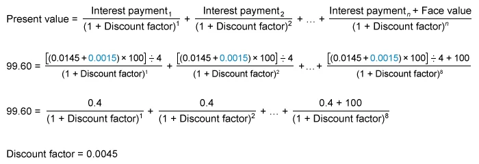
The price of an FRN is its discounted future payments, where the discount factor is based on the reference rate plus a discount margin. The discount margin represents the market’s required spread to price the FRN at par on the reset date.
To solve for the discount margin, first calculate the discount factor and then use that to derive the discount margin.
- Calculate the discount factor (using a financial calculator):
-
Use the discount factor to find the discount margin:
(Choice B) 40 bps is the difference between the market price and par value, not the discount margin.
(Choice C) 45 bps is the periodic discount factor, not the discount margin. The periodic discount factor equals the sum of the reference rate and the discount margin (180 bps) divided by the number of periods per year (4).
Things to remember:
A floating-rate note (FRN) is a debt instrument with an interest rate that resets periodically and is based on a reference rate, such as LIBOR, plus a quoted margin. The price of an FRN is its discounted future payments, where the discount factor is based on the reference rate plus a discount margin that reflects the market’s required return.
A coupon bond’s Macaulay duration is most accurately described as the holding period over which:
- the value of cash flows received equal the cost of buying the bond.
- changes in reinvestment income offset changes in the bond’s price.
- the bond earns a risk-free return if hedged by shorting a government bond.
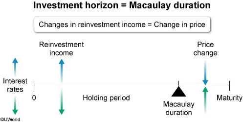
Noncallable coupon bonds contain two types of interest rate risk: reinvestment risk and price risk. Reinvestment risk dominates in the long run and price risk dominates in the short run. Logically, somewhere in between the short run and the long run, there should be a balance point. That point is the Macaulay duration: the holding period to the point where changes in reinvestment income and changes in price offset one another exactly.
- Interest rates increase: additional reinvestment income and bond price decreases
- Interest rates decrease: reduced reinvestment income and bond price increases
No matter the direction, the impact of a rate change is positive for one source of return, but negative for the other. In the short run, price risk dominates. Interest rate changes affect bond prices immediately. In the long run, reinvestment risk dominates since its impact builds over time as more coupons are reinvested. A bond’s Macaulay duration is the holding period over which those risks balance each other.
(Choice A) Market price equals the present value of the coupon and principal, so a bond must be held to maturity to receive cash flows with a value equal to the cost of the bond. Since Macaulay duration is the present value weighted average time of the cash flows, a coupon bond’s Macaulay duration is shorter than its time to maturity.
(Choice C) Although it is a type of hedge, the strategy is not riskless and therefore does not lock in a risk-free rate of return.
Things to remember:
The Macaulay duration is the holding period of a bond to the point where changes in reinvestment income and changes in price offset one another exactly.
What to Expect in CFA Level 2 Fixed Income
The CFA Level 2 Fixed Income is one of the most heavily weighted topics on the exam. The material introduces traditional and modern theories regarding the shape of the yield curve and the fundamental relationships underpinning its composition. You will study valuation methods used to value bonds with embedded options and various credit analysis concepts.
Exam Weight
The CFA Fixed Income topic has a weight of 10-15% of the total exam content, so that approximately 8-12 questions or 2-3 item sets on the CFA Level 2 exam focus on this topic.
| No. of Readings | No. of Formulas |
|---|---|
| 5 | ca. 60 |
Level 2 Fixed Income Syllabus, Readings, and Changes
The CFA Level 2 curriculum includes 5 learning modules for the Fixed Income topic (10% of the total curriculum). There have been only minor updates to the L2 Fixed Income curriculum.
| No. of Learning Modules – 5 | No. of LOS – 50 | |
|---|---|---|
Summary These learning modules focus on the following categories of Alternative Investments: real estate, private equity, and commodities. The Fixed Income curriculum introduces the yield curve and fundamental aspects of its composition. You will learn various theories regarding yield curve shape and an arbitrage-free framework for valuing option-free bonds. It then builds on binomial valuation methods to value bonds with embedded options. You will study credit analysis, the term structure of credit spreads, and how credit default swaps are used in managing credit exposure. | ||
The Term Structure and Interest Rate Dynamics
Interest rates act to influence and measure the economy. Quantifying interest rate risk is an important skill for risk managers, and understanding the determinants of interest rates is important for issuers of and investors in fixed-income securities.
The learning module explains spot rates and forward rates and their influence on the yield curve shape. You will build on this information to understand how forward rates influence the yield-to-maturity and expected bond returns.
The Arbitrage-Free Valuation Framework
Valuing fixed income securities, derivatives, and other financial assets is predicated on the idea that market prices adjust until arbitrage opportunities expire
The learning module introduces concepts and techniques for no-arbitrage valuation of Fixed Income securities. This includes discussions of the binomial interest rate tree and a Monte Carlo forward-rate simulation.
Valuation and Analysis of Bonds with Embedded Options
The value of embedded options is typically contingent on interest rates. This makes bond valuation more complex when a bond has one or more embedded options. Bond issuers and investors must understand how various embedded options influence bond values and their sensitivity to interest rate changes.
The learning module introduces a summary of different types of embedded options before exploring bonds that include a call or put provision. You will also learn about how option-adjusted spreads are used to value risky callable and putable bonds.
Credit Analysis Models
Credit analysis models rely on inputs such as exposure to default loss, the loss given default, and the probability of default. These models are an important part of valuing corporate and government bonds.
You are introduced to structural and reduced-form credit analysis models. The learning module also covers the arbitrage-free framework and compares the credit analysis for securitized debt with that of corporate bonds.
Credit Default Swaps
A credit default swap is a financial contract between 2 parties that enables an investor to “swap” or offset credit risk with another investor for a defined period of time. These derivative instruments are broadly used internationally.
The learning module classifies these instruments and explores their fundamental concepts. You will learn about the elements associated with their valuation, pricing, and applications.
CFA Fixed Income Level 2 Sample Questions and Answers
These sample questions are typical of the L2 exam’s complexity and depth – formatted as item sets, with a vignette to deliver a scenario that tests the CFA L2 curriculum. On the actual exam, each vignette applies to 4 questions. We’ve added a few additional questions for you to practice with. Be sure to review the illustrated explanations we’ve provided for each question. UWorld’s question bank is designed to expose you to exam-like questions and explain the concepts tested thoroughly.
Which of the three approaches for the arbitrage-free valuation of option-free bonds described by Muon is least likely correct?
- Approach 1
- Approach 2
- Approach 3
Approach 1: Value the bond as a portfolio of zero-coupon bonds that replicate the bond’s cash flows.
Approach 2: Value the bond as the sum of the individual cash flows’ present values, discounting each cash flow by the spot rate with a matching term.
Approach 3: Value the bond as the sum of the individual cash flows’ present values, discounting each cash flow by the YTM of a benchmark bond with the same time to maturity as the bond.
Arbitrage-free valuation of option-free bonds is based on the no-arbitrage principle: market prices adjust until there is no possibility of making risk-free profits through the simultaneous purchase and sale of related assets. This principle is based on two related, fundamental concepts.
- The law of one price: Assets that are perfect substitutes (eg, same asset traded in different markets, an asset and its related forward contract) must trade at equivalent values.
- Value additivity: The value of the whole must equal the sum of the value of its parts.
The arbitrage-free pricing of a coupon bond reflects these concepts by discounting individual cash flows by the spot rate with a term that matches the bond’s payment dates (Choice B). This approach values the bond as a portfolio of zero-coupon bonds that replicate the amount and timing of the bond’s coupons and principal (Choice A). As a result, each discount rate incorporates any risks captured in market term premiums.
Discounting a coupon bond’s cash flows by a single rate (as suggested in Approach 3) is inappropriate for estimating the bond’s arbitrage-free value—unless the yield curve is flat, which is clearly not the case in this instance (Exhibits 1 and 2). If the single discount rate were the bond’s YTM, the result would be the bond’s market price, which could never reveal an arbitrage opportunity. In addition, a single rate would not reflect any difference in risk (eg, expected inflation) from the variation of interest rates across maturities.
Things to remember:
The arbitrage-free valuation of option-free bonds is based on value additivity and the law of one price. These two concepts are applied to a coupon bond by discounting the bond’s individual cash flows by the appropriate-term spot rate. This treats the bond as a portfolio of zero-coupon bonds that match the amount and timing of the bond’s coupons and principal.
Based on Exhibits 1 and 2, which bond has a market price that best reflects its arbitrage-free price?
- Bond A
- Bond B
- Bond C
| Exhibit 1 US Benchmark Par Curve Bonds | |
|---|---|
| Maturity (years) | YTM |
| 1 | 1.50% |
| 2 | 2.00% |
| 3 | 2.50% |
| Exhibit 2 Summary Data for US 3-Year Bonds | ||
|---|---|---|
| Coupon rate | Market price | |
| Bond A | 2.50% | 100.251 |
| Bond B | 3.00% | 101.737 |
| Bond C | 3.50% | 102.847 |
P0 =
P0 = Arbitrage-free price
PMT = Periodic coupon
r ( J ) = J – period spot rate
The arbitrage-free value of a coupon bond is the sum of the present value of the bond’s cash flows discounted by the appropriate-term spot rates. Violations of the no-arbitrage principle are uncovered by comparing a bond’s arbitrage-free value, based on a spot rate curve, to the bond’s market price, based on a single discount rate (ie, the bond’s YTM).
1 =
PBCN = Par bond coupon for bond with N years to maturity
r ( J ) = J – period spot rate
N = Number of periods to maturity
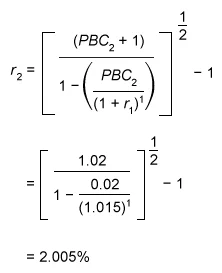
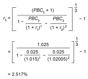
Spot rates are bootstrapped from a benchmark (eg, government bond) par yield curve. Bootstrapping is an iterative process that extends a spot rate curve one period at a time. Each iteration uses a par bond with a maturity equal to the term of the spot rate being calculated.
A par bond has a price of 1.00 (ie, 100% of par) and a coupon rate equal to its YTM. Each cash flow before maturity is discounted by the (previously calculated) appropriate-term spot rate. The cash flows are known, as are all spot rates except the one for the final period. Using the bootstrapping equation from above, solve for the final-period discount rate, which is the spot rate for a term matching the bond’s maturity.
The 1-year spot rate is equal to the 1-year par rate: 1.50%.
The 2-year spot rate is calculated by rearranging the equation as follows:
The 3-year spot rate is calculated as follows:
Use the spot rates bootstrapped from the par bond rates to calculate the arbitrage-free values of the bonds. However, note that Bond A requires no calculation: since the bond has a coupon rate equal to the 3-year par bond YTM, it has an arbitrage-free value equal to 100% of par.
| Arbitrage-free value | Market price | |
|---|---|---|
| Bond A |
2.5
/
(1.015) 1
+
2.5
/
(1.02005) 2
+
102.5
/
(1.02517) 3
= 100.000
|
100.251 |
| Bond B |
3.0
/
(1.015) 1
+
3.0
/
(1.02005) 2
+
103.0
/
(1.02517) 3
= 101.437
|
101.737 |
| Bond C |
3.5
/
(1.015) 1
+
3.5
/
(1.02005) 2
+
103.5
/
(1.02517) 3
= 102.874
|
102.847 |
Things to remember:
The arbitrage-free value of a coupon bond is the sum of the present value of the bond’s cash flows discounted by the appropriate-term spot rates. The spot rates for an arbitrage-free valuation can be bootstrapped from a par bond curve.
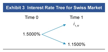
Based on Exhibit 3, if Muon assumes a volatility of 20%, the interest rate at the higher-rate node at Time 1 is closest to:
- 1.40%
- 1.72%
- 3.13%
Binomial interest rate trees are based on a benchmark yield curve. For all periods beyond Time 0, the tree consists of 1-period forward rates, which are calculated through a trial-and-error process using:
- a benchmark bond maturing one period beyond the previously obtained rates,
- an assumed volatility that is the same for the entire tree,
- the benchmark yield curve 1-period spot rate, and
- 1-period forward rates obtained from all previous iterations of this process.
Binomial rate tree construction requires assumptions about how interest rates change. The standard approach is to assume interest rate changes are lognormally distributed. This assumption leads to the relationship between the rates at adjacent nodes at a given period of time, as shown in this tree. To calculate the 1-period higher forward rate, use the 1-period lower forward rate (i1,L) and the given volatility (20%).
| i1,H | = i1,L × e2σ |
| = 0.0115 × e2(0.2) | |
| = 0.0115 × 1.492 | |
| = 1.72% |
Note: The “lower” rate one period in the future is not necessarily below the interest rate at the previous node; it is lower relative to the “higher” rate for that period. Depending on the slope of the benchmark spot rate curve, the “lower” rate at the next period could be either above or below the interest rate at the preceding node.
(Choice A) 1.40% results from multiplying i1,L by e2, which fails to reflect that the exponent is 2 times the volatility.
(Choice C) 3.13% results from multiplying i1,L by e, which is incorrect since e must be raised to the power of 2 times the volatility.
Things to remember:
Rates on a binomial interest rate tree are calculated through a trial-and-error process, using benchmark bonds and an assumed volatility. For two adjacent nodes at a given time period, the higher rate is derived from the lower interest rate and the assumed volatility.
What to Expect in CFA Level 3 Fixed Income?
Fixed Income is no longer a stand-alone topic at Level 3, but it is heavily integrated into Portfolio Management. Bond valuation concepts, yield curve dynamics, interest rate risk, and liability-driven investing all reappear inside PM and Wealth Management readings.
Frequently Asked Questions (FAQs)
Is CFA Level 1 Fixed Income hard?
CFA Level 1 Fixed Income is considered 1 of the more difficult topics on the exam. For most students, it is also 1 of the least familiar. Fixed-income securities are typically more abstract than equity investments. It’s likely you are more familiar with the stock exchange and equity investments than you are with debt securities.
The earning modules are highly theoretical and laden with novel terms. You are introduced to several bond valuation methods and complicated concepts related to risk and return analysis. However, having a solid understanding of Fixed Income is critical to the CFA charter.
Is the CFA Level 2 Fixed Income topic hard?
Like its Level 1 counterpart, the CFA Level 2 Fixed Income is considered 1 of the more difficult topics on the exam. Fixed income is relatively heavy on formulas and theory. You will study various formulae used to value bonds with embedded options and the theoretical and practical aspects of the yield curve.
What topics are included in the CFA Fixed Income syllabus?
The Fixed Income syllabus includes bond features and types, pricing and yield measures, interest rate risk, duration and convexity, credit risk, securitization, the term structure of interest rates, yield curve dynamics, and, at Level 2, valuation of bonds with embedded options, credit analysis, structured products, and multi-factor interest rate models.
How many Fixed Income questions appear on the CFA exam?
Fixed Income typically represents 10–12% of the Level 1 exam, which is roughly 18–22 questions, and about 10–15% of the Level 2 exam, which corresponds to one to three item sets depending on the exam cycle.
What is the difference between Fixed Income in Level 1 and Level 2?
Level 1 focuses on bond basics, pricing, yields, duration, convexity, and introductory risk concepts, while Level 2 expands into advanced valuation techniques, yield curve modeling, credit analysis, structured securities, and bonds with embedded options, requiring deeper interpretation and more quantitative analysis.
Does Fixed Income appear as a stand-alone topic in CFA Level 3?
Fixed Income does not appear as a stand-alone topic at Level 3, but its concepts including interest rate expectations, bond portfolio strategies, credit exposures, and duration management are heavily integrated into the Portfolio Management and Wealth Management curriculum.
Which Fixed Income topics are considered the hardest?
The most challenging topics include valuation of bonds with embedded options, multi-factor interest rate models, credit risk modeling, mortgage-backed securities, securitization, and duration/convexity calculations due to their quantitative and conceptual complexity.
Is Fixed Income formula-heavy?
Yes. Fixed Income relies on numerous formulas for bond pricing, yield calculations, duration, convexity, spot rate extraction, forward rates, and option-adjusted spread analysis, making it one of the more mathematically intensive topics on the CFA exams.
What formulas are most important in CFA Fixed Income?
Key formulas include present value of bond cash flows, yield to maturity, spot and forward rate calculations, Macaulay and modified duration, convexity, effective duration for bonds with embedded options, and spread measures such as G-spread, I-spread, Z-spread, and option-adjusted spread (OAS).
How should I study Fixed Income for the CFA exam?
The best approach is to build a solid understanding of core pricing and yield concepts, practice duration and convexity problems, work through bond valuation examples, and use QBanks and mock exams to improve speed and accuracy, as Fixed Income questions often require multiple calculation steps.


